For Christopher Costello costello@bren.ucsb.edu, facilitated by Reniel Cabral rcabral@bren.ucsb.edu.
Install bbnj R package
Install the bbnj R package (and devtools if needed).
install.packages(devtools)
devtools::install_github("ecoquants/bbnj")
Get Data
See list of datasets in bbnj reference. Datasets are “lazy-loaded”" with library(bbnj), meaning available in path but not showing up in Environment tab of RStudio.
library(tidyverse)
library(raster)
library(bbnj)

# list bbnj datasets in RStudio:
data(package="bbnj")

# list raster layers within stacks (s_*)
names(s_fish_gfw)
## [1] "fishing_KWH"
## [2] "mean_costs"
## [3] "revenue"
## [4] "mean_scaled_profits"
## [5] "mean_scaled_profits_with_subsidies"
## [6] "scaled_profits_low_labor_cost"names(s_bio_gmbi)## [1] "nspp_all_2100" "nspp_all"
## [3] "nspp_bivalves_2100" "nspp_bivalves"
## [5] "nspp_chitons_2100" "nspp_chitons"
## [7] "nspp_coastal.fishes_2100" "nspp_coastal.fishes"
## [9] "nspp_corals_2100" "nspp_corals"
## [11] "nspp_crustaceans_2100" "nspp_crustaceans"
## [13] "nspp_echinoderms_2100" "nspp_echinoderms"
## [15] "nspp_euphausiids_2100" "nspp_euphausiids"
## [17] "nspp_gastropods_2100" "nspp_gastropods"
## [19] "nspp_hydrozoans_2100" "nspp_hydrozoans"
## [21] "nspp_na_2100" "nspp_na"
## [23] "nspp_non.squid.cephalopods_2100" "nspp_non.squid.cephalopods"
## [25] "nspp_pinnipeds_2100" "nspp_pinnipeds"
## [27] "nspp_reptiles_2100" "nspp_reptiles"
## [29] "nspp_sea.spiders_2100" "nspp_sea.spiders"
## [31] "nspp_seagrasses_2100" "nspp_seagrasses"
## [33] "nspp_sharks_2100" "nspp_sharks"
## [35] "nspp_sponges_2100" "nspp_sponges"
## [37] "nspp_tunas.n.billfishes_2100" "nspp_tunas.n.billfishes"
## [39] "nspp_tunicates_2100" "nspp_tunicates"
## [41] "nspp_worms_2100" "nspp_worms"
## [43] "rls_all_2100" "rls_all"
## [45] "rls_bivalves_2100" "rls_bivalves"
## [47] "rls_coastal.fishes_2100" "rls_coastal.fishes"
## [49] "rls_corals_2100" "rls_corals"
## [51] "rls_echinoderms_2100" "rls_echinoderms"
## [53] "rls_na_2100" "rls_na"
## [55] "rls_non.squid.cephalopods_2100" "rls_non.squid.cephalopods"
## [57] "rls_pinnipeds_2100" "rls_pinnipeds"
## [59] "rls_reptiles_2100" "rls_reptiles"
## [61] "rls_sharks_2100" "rls_sharks"
## [63] "rls_tunas.n.billfishes_2100" "rls_tunas.n.billfishes"# get rasters from stacks
profit_fishing <- raster(s_fish_gfw, "mean_scaled_profits_with_subsidies") %>%
gap_fill_raster()
nspp_tunas <- raster(s_bio_gmbi, "nspp_tunas.n.billfishes")
nspp_sharks <- raster(s_bio_gmbi, "nspp_sharks")
# stack wanted rasters for later cropping
s <- stack(profit_fishing, nspp_tunas, nspp_sharks)
names(s) <- c("profit_fishing", "nspp_tunas", "nspp_sharks")Get Area of Interest
You’ll need to run the raster::drawExtent() function interactively (ie not “knitting”) within RStudio, outputting to console.
aoi_rds   <-   "aoi.rds"
s_aoi_rds <- "s_aoi.rds"

if (interactive()){
  # draw your own area of interest
  plot(nspp_tunas)
  aoi <- raster::drawExtent()
  saveRDS(aoi, file = aoi_rds)
} else {
  # load existing
  aoi <- readRDS(aoi_rds)
}

# show area of interest
aoi
## class : Extent
## xmin : -6.523557
## xmax : 23.58517
## ymin : -46.54307
## ymax : -26.47059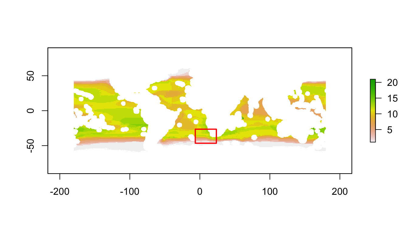
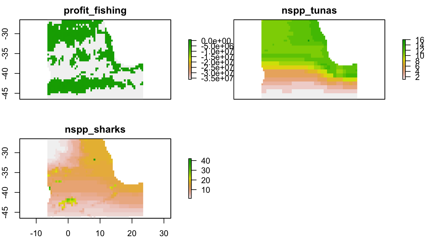
# crop raster
s_aoi <- raster::crop(s, aoi)

# save and plot
saveRDS(s_aoi, file = s_aoi_rds)
plot(s_aoi)